Subset interaction effect

Introduction

In omics research frameworks like limma are gold standard to test for differetnial expressed genes. However inbalances of the input data might increase the FPR of such linear models. A subset approach should mitigate this problem.

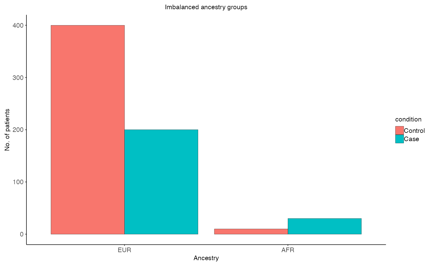
Overrepresentation of EUR ancestry

In omics research EUR ancestry is often overrepresented compared to other ancestries. Hence, data of non-Europeans is often sparse and can effect the discovery of true effects. The frameworkCrossAncestryGenPhen tries to be fair by subsampling the overrepresented ancestry to match the sample size of the underrepresented ancestry. The following code snippet showcases such an imbalance on a simulated dataset.

library(CrossAncestryGenPhen)

# Seed for reproducibility
set.seed(42)

# Example data 
n_features <- 100  
n_EUR <- 600 
n_AFR <- 40  

id_EUR <- paste0("EUR_", seq_len(n_EUR))
id_AFR <- paste0("AFR_", seq_len(n_AFR))

lambda_features <- sample(
  c(
    rpois(20, 3),    # ~20 low-count features
    rpois(60, 20),   # ~60 medium-count features
    rpois(20, 120)   # ~20 high-count features
  ),
  size = n_features,
  replace = FALSE
)

# Expression matrices for EUR and AFR ancestries
X <- sapply(lambda_features, function(lam) rpois(n_EUR, lambda = lam))
Y <- sapply(lambda_features, function(lam) rpois(n_AFR, lambda = lam))
colnames(X) <- colnames(Y) <- paste0("Feature_", seq_len(n_features))


# Metadata for EUR and AFR ancestries
# EUR: overrepresented compared to AFR
MX <- data.frame(
  condition = factor(c(rep("Control", 400), rep("Case", 200)), levels = c("Control", "Case")),
  ancestry = "EUR",
  sex      = sample(c("Male", "Female"), n_EUR, replace = TRUE),
  age      = round(rnorm(n_EUR, mean = 50, sd = 12))
)

# AFR: underrepresented compared to EUR
MY <- data.frame(
  condition = factor(c(rep("Control", 10), rep("Case", 30)), levels = c("Control", "Case")),
  ancestry = "AFR",
  sex      = sample(c("Male", "Female"), n_AFR, replace = TRUE),
  age      = round(rnorm(n_AFR, mean = 48, sd = 11))
)

# Rownames of matrix must be smaple ids
rownames(X) <- rownames(MX) <- id_EUR
rownames(Y) <- rownames(MY) <- id_AFR


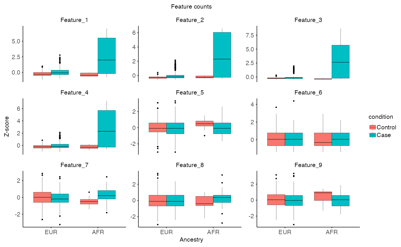
# Spike in effect in AFR Case (strong effect, but only for half of AFR cases)
# AFR Case: strong effect, half of cases
afr_case_idx <- which(MY$condition == "Case")
afr_spike_idx <- sample(afr_case_idx, length(afr_case_idx) / 2)
Y[afr_spike_idx, 1:4] <- Y[afr_spike_idx, 1:4] +
  rpois(length(afr_spike_idx) * 4, lambda = 80)

# EUR Case: weaker effect, 20% of cases
eur_case_idx <- which(MX$condition == "Case")
eur_spike_idx <- sample(eur_case_idx, length(eur_case_idx) * 0.2)
X[eur_spike_idx, 1:4] <- X[eur_spike_idx, 1:4] +
  rpois(length(eur_spike_idx) * 4, lambda = 20)

# Plot imbalance
plot_imbalanced_groups(
  MX = MX,
  MY = MY,
  x_var = "ancestry",
  fill_var = "condition",
  title = "Imbalanced ancestry groups",
  x_label = "Ancestry",
  y_label = "No. of patients"
)

# Plot features
plot_feature(
  X = X, 
  Y = Y, 
  MX = MX, 
  MY = MY, 
  x_var = "ancestry",
  fill_var = "condition",
  title = "Feature counts",
  x_label = "Ancestry",
  y_label = "Z-score"
)

Sample imbalance

Contrasts in `limma_interaction_effect`

The function limma_interaction_effect() fits a 2 × 2 design (two groups × two ancestries) and evaluates four main contrasts plus the interaction.
Here is a summary of what each contrast represents:

Coef type	Formula	Interpretation
baseline_1	`G1.A2 – G1.A1`	Ancestry effect (A2 vs. A1) within group G1.
baseline_2	`G2.A2 – G2.A1`	Ancestry effect (A2 vs. A1) within group G2.
relationship_1	`G2.A1 – G1.A1`	Group effect (G2 vs. G1) within ancestry A1.
relationship_2	`G2.A2 – G1.A2`	Group effect (G2 vs. G1) within ancestry A2.
interaction	`(G2.A2 – G1.A2) – (G2.A1 – G1.A1)`	Does the group effect differ by ancestry? (group × ancestry interaction).

G1 / G2 = the two levels of your g_col variable (e.g. Control / Case).
A1 / A2 = the two ancestries provided (MX == A1 and MY == A2).

res <- limma_interaction_effect(
  X = X,
  Y = Y,
  MX = MX,
  MY = MY,
  g_col = "condition",
  a_col = "ancestry",
  covariates = c("sex", "age"),
  use_voom = TRUE,
  verbose = TRUE
)
#> 
#> Linear model summary:
#> Formula:        ~0 + groups + sex + age
#> Groups:         Control.EUR  Case.EUR  Control.AFR  Case.AFR
#> Baseline:       Control.AFR - Control.EUR  Case.AFR - Case.EUR
#> Relationship:   Case.EUR - Control.EUR  Case.AFR - Control.AFR
#> Interaction:    (Case.AFR - Control.AFR) - (Case.EUR - Control.EUR)

print(head(res))
#>    coef_type                  contrast   feature       T_obs   p_value
#> 1 baseline_1 Control.AFR - Control.EUR Feature_1 -0.10683710 0.5296430
#> 2 baseline_1 Control.AFR - Control.EUR Feature_2  0.18229653 0.6783480
#> 3 baseline_1 Control.AFR - Control.EUR Feature_3 -0.66960349 0.2858098
#> 4 baseline_1 Control.AFR - Control.EUR Feature_4 -0.03846892 0.8395951
#> 5 baseline_1 Control.AFR - Control.EUR Feature_5  0.15718092 0.1140348
#> 6 baseline_1 Control.AFR - Control.EUR Feature_6 -0.10661937 0.7439013
#>       p_adj  ave_expr
#> 1 0.8682672 12.618695
#> 2 0.9311933 10.371654
#> 3 0.8682672  9.929222
#> 4 0.9433653 12.358806
#> 5 0.8682672 12.407350
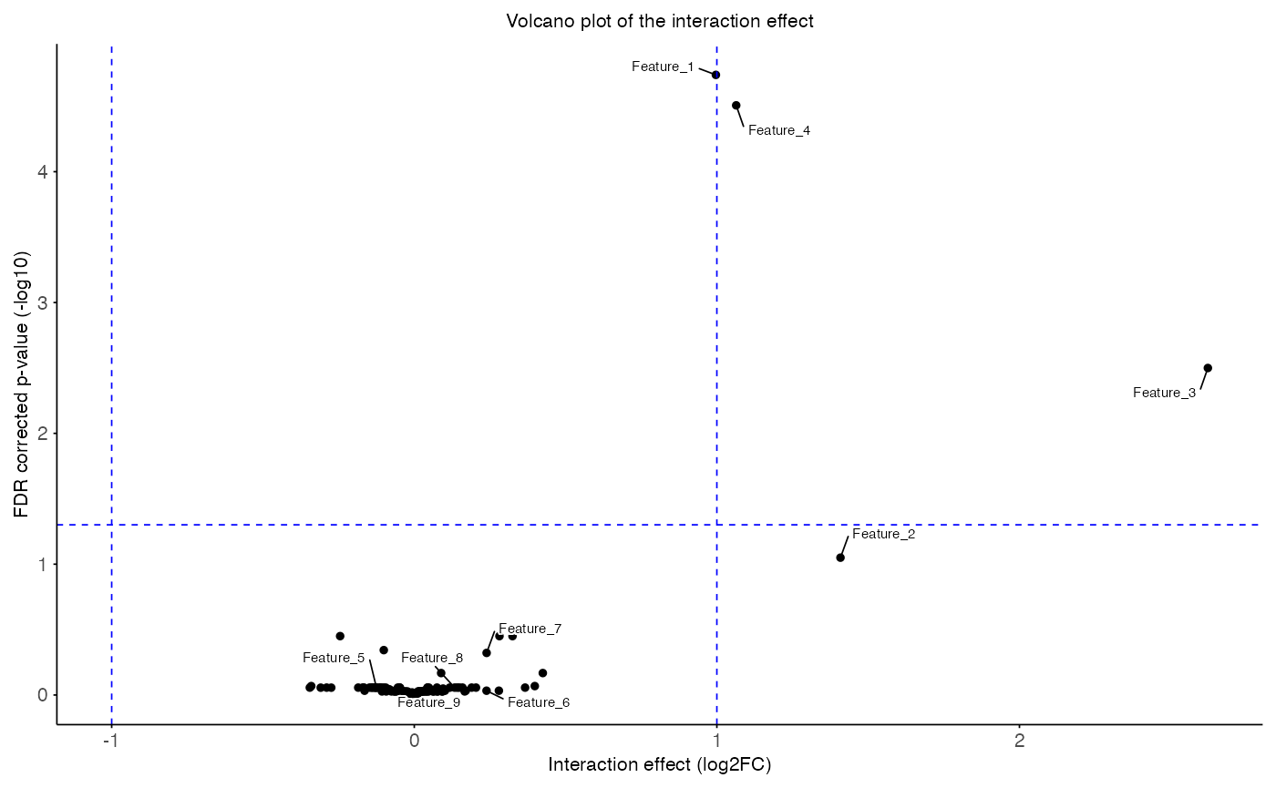
#> 6 0.9311933  9.058603

The output can easily be filtered for the coefficient of interest and plotted with the function plot_volcano().

# Filter for interaction effect
interaction_res <- subset(res, coef_type == "interaction")

plot_volcano(
  data = interaction_res, 
  x_var = "T_obs", 
  y_var = "p_adj", 
  sig_thr = 0.05, 
  effect_thr = 1,
  features = head(interaction_res$feature, 9),
  title = "Volcano plot of the interaction effect", 
  x_label = "Interaction effect (log2FC)",
  y_label = "FDR corrected p-value (-log10)"
)

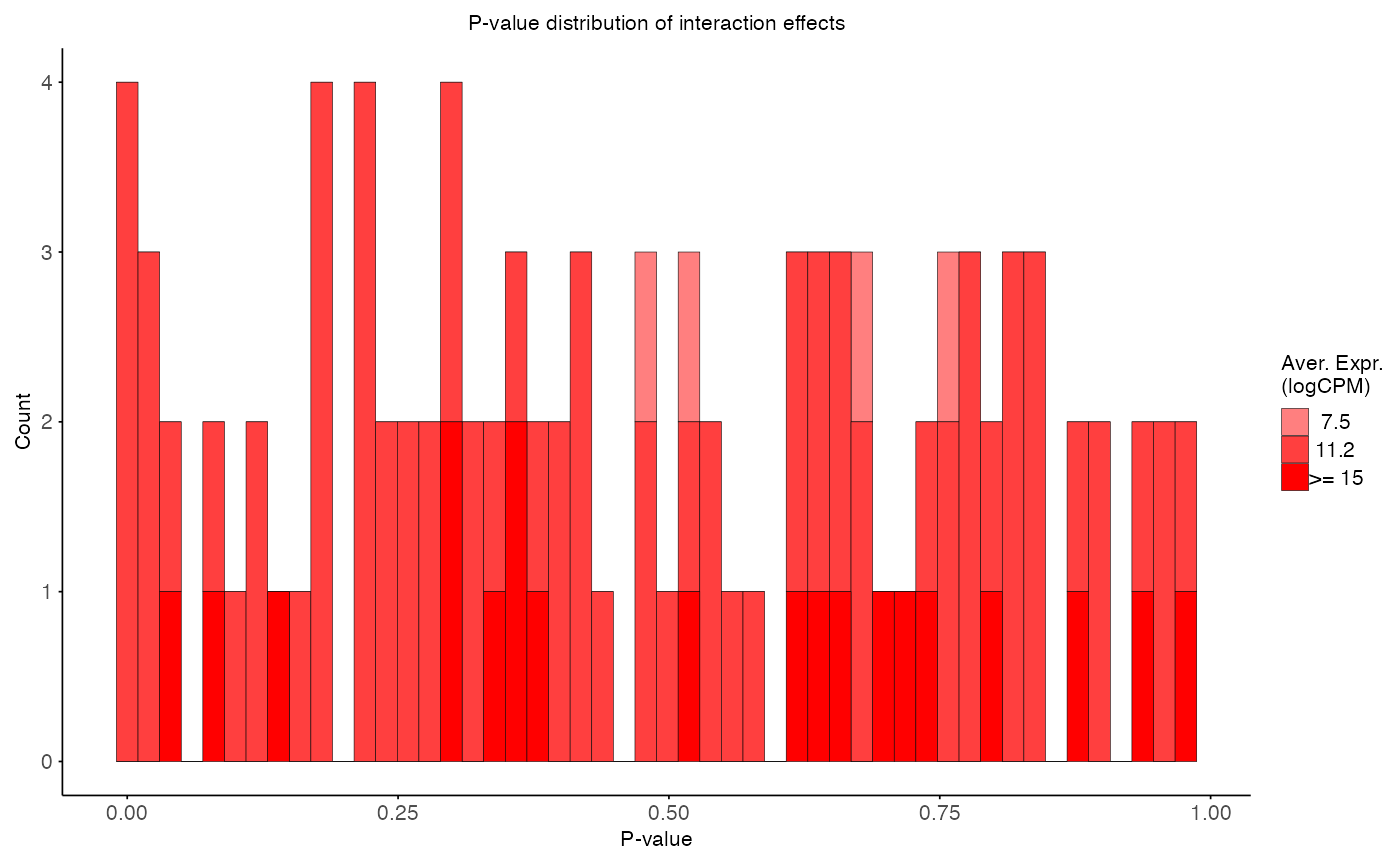
plot_pvalue_distribution(
  data = interaction_res,
  x_var = "p_value",
  fill_var = "ave_expr",
  facet_col = NULL,
  facet_levels = NULL,
  title = "P-value distribution of interaction effects",
  x_label = "P-value",
  y_label = "Count",
  fill_label = "Aver. Expr.\n(logCPM)"
)

Volcano plot

Assuming we found significant

Single subset run

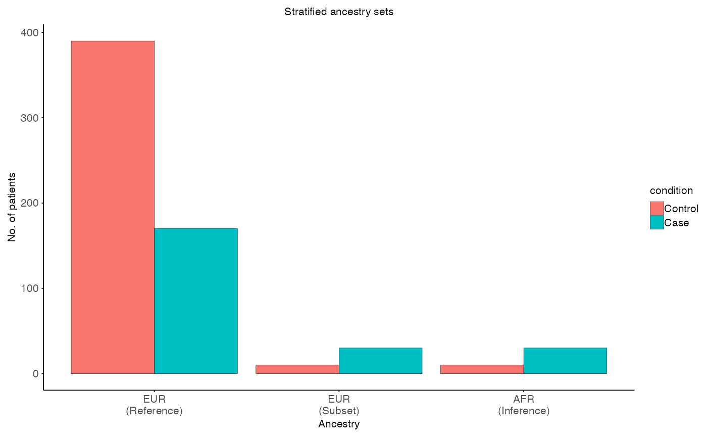
Stratification step

The function split_stratified_ancestry_sets creates a stratified subset to account for sample size but also control for the phenotype imbalance in the underrepresented ancestry. The idea is to create a EUR Train-set, which is the remaining EUR cohort after subsampling, a EUR-subset Test-set (mimicking the underrepresented ancestry) based on the compared ancestry Inferecnce-set. The function plot_stratified_sets plots the stratified ancestry sets. 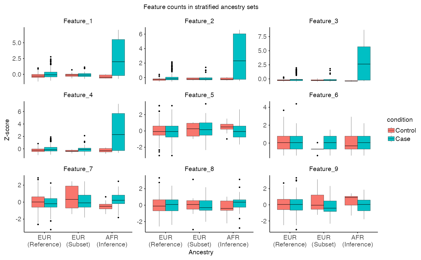The function plot_stratified_feature allows to plot single or multiple features per split.


# Split the data into stratified sets
split <- split_stratified_ancestry_sets(
  X = X,
  Y = Y,
  MX = MX,
  MY = MY,
  g_col = "condition",
  a_col = "ancestry",
  seed = 42,
  verbose = TRUE
)
#> 
#> Stratified split summary:
#> EUR (Reference, R):    N: 560  Control: 390  Case: 170
#> EUR (Subset, X):       N: 40   Control: 10   Case: 30
#> AFR (Inference, Y):    N: 40   Control: 10   Case: 30

# Visulaize stratified sets
plot_stratified_sets(
  MX = split$X$meta,
  MY = split$Y$meta,
  MR = split$R$meta,
  x_var = "ancestry",
  fill_var = "condition",
  title = "Stratified ancestry sets",
  x_label = "Ancestry",
  y_label = "No. of patients"
)

# Visulaize stratified features
plot_stratified_feature(
  X = split$X$counts,
  Y = split$Y$counts,
  R = split$R$counts,
  MX = split$X$meta,
  MY = split$Y$meta,
  MR = split$R$meta,
  x_var = "ancestry",
  fill_var = "condition",
  title = "Feature counts in stratified ancestry sets",
  x_label = "Ancestry",
  y_label = "Z-score"
)

Sample balance

Limma interaction effect on single subset

The function split_stratified_ancestry_sets creates on subset of the overrepresented ancestry. Note: A single subset only generates one estimate of the difference it is recomendet to run multiple subsets to get a more robust estimate of the interaction effect.

res <- limma_interaction_effect(
  X = split$X$counts,
  Y = split$Y$counts,
  MX = split$X$meta,
  MY = split$Y$meta,
  g_col = "condition",
  a_col = "ancestry",
  covariates = c("sex", "age"),
  use_voom = TRUE,
  verbose = TRUE
)
#> 
#> Linear model summary:
#> Formula:        ~0 + groups + sex + age
#> Groups:         Control.EUR  Case.EUR  Control.AFR  Case.AFR
#> Baseline:       Control.AFR - Control.EUR  Case.AFR - Case.EUR
#> Relationship:   Case.EUR - Control.EUR  Case.AFR - Control.AFR
#> Interaction:    (Case.AFR - Control.AFR) - (Case.EUR - Control.EUR)

res <- subset(res, coef_type == "interaction")

print(head(res))
#>       coef_type                                            contrast   feature
#> 401 interaction (Case.AFR - Control.AFR) - (Case.EUR - Control.EUR) Feature_1
#> 402 interaction (Case.AFR - Control.AFR) - (Case.EUR - Control.EUR) Feature_2
#> 403 interaction (Case.AFR - Control.AFR) - (Case.EUR - Control.EUR) Feature_3
#> 404 interaction (Case.AFR - Control.AFR) - (Case.EUR - Control.EUR) Feature_4
#> 405 interaction (Case.AFR - Control.AFR) - (Case.EUR - Control.EUR) Feature_5
#> 406 interaction (Case.AFR - Control.AFR) - (Case.EUR - Control.EUR) Feature_6
#>          T_obs    p_value     p_adj  ave_expr
#> 401  1.2186459 0.01163693 0.5036107 12.970857
#> 402  1.9562581 0.09064993 0.5036107 11.104253
#> 403  3.0480689 0.03312673 0.5036107 10.577955
#> 404  1.0454901 0.07158428 0.5036107 12.696330
#> 405 -0.1412233 0.35553674 0.8228834 12.451729
#> 406 -0.2792438 0.57859836 0.8358211  9.023236

Multiple subset runs

As mentioned, a single subset only generates one estimate of the difference. To get a more robust estimate of the interaction effect, it is recommended to run multiple subsets. In this case the pipeline is similar to run a single subset but with concerns on how to aggregate over multiple subsets. Because the samples from the underrepresented ancestry are identical over multiple subsets this introduced dependence. Hence, aggregating p-values or test statistics is not trivial.

# We track the SampleIDs and the summary statisitcs over many subsets
res_log <- list()
id_log  <- list()

for (i in 1:10) {
  
  # Stratified ancestry sets
  split <- split_stratified_ancestry_sets(
    X = X,
    Y = Y,
    MX = MX,
    MY = MY,
    g_col = "condition",
    a_col = "ancestry",
    seed = 42 + i,
    verbose = FALSE
  )

  # Store sample ids
  id_log[[i]] <- track_sample_ids(split, i)

  # Limma interaction effects
  res <- limma_interaction_effect(
    X = split$X$counts,
    Y = split$Y$counts,
    MX = split$X$meta,
    MY = split$Y$meta,
    g_col = "condition",
    a_col = "ancestry",
    covariates = c("sex", "age"),
    use_voom = TRUE,
    verbose = FALSE
  )

  res <- subset(res, coef_type == "interaction")


  # Store subset runs
  res$iteration <- i
  res_log[[length(res_log) + 1]] <- res
}

# Combine across iterations
combined_res <- do.call(rbind, res_log)
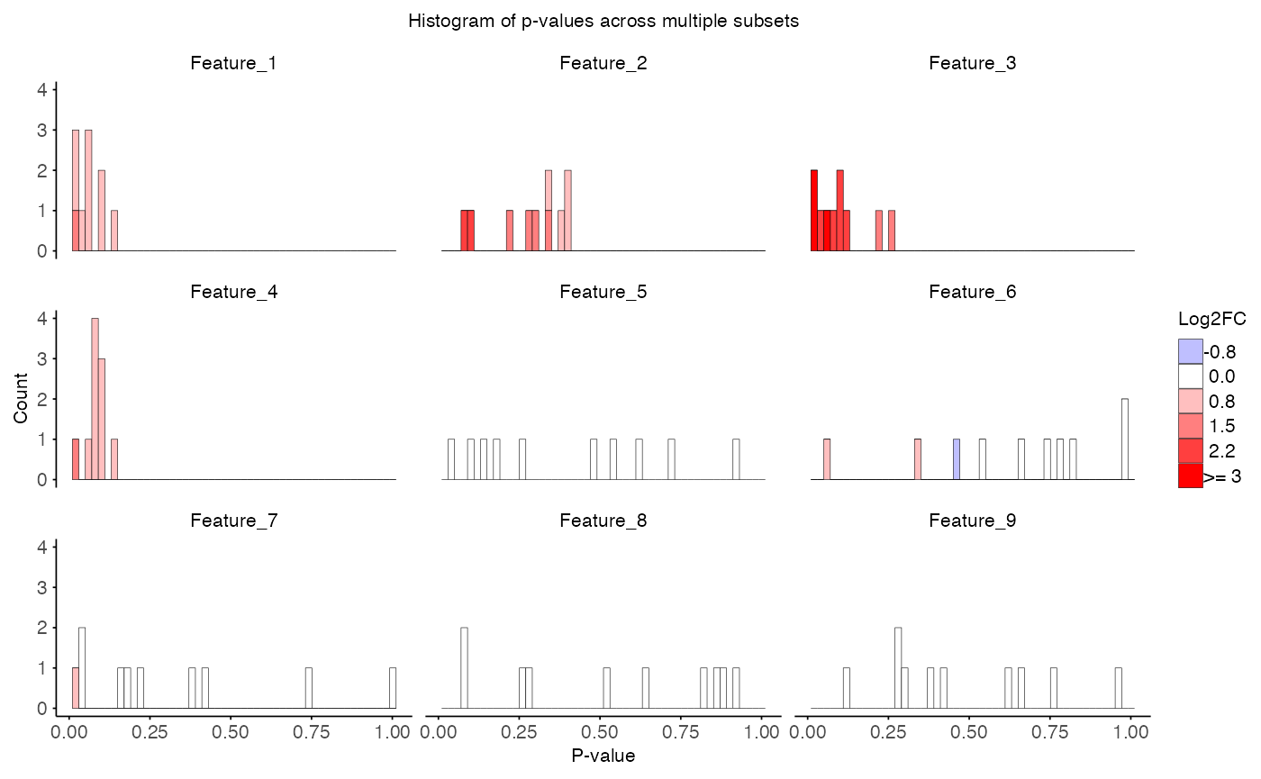
combined_id  <- do.call(rbind, id_log)

With this loop we calculated the interaction effect over many subsets. Hence, we have a p-value for each feature in each subset. We can plot this distribution of p-values with the function plot_pvalue_distribution().

# Visualize p-value distribution
plot_pvalue_distribution(
  data = combined_res,
  x_var = "p_value",
  fill_var = "T_obs",
  facet_col = "feature",
  title = "Histogram of p-values across multiple subsets",
  x_label = "P-value",
  y_label = "Count",
  fill_label = "Log2FC",
  bins = 50,
  fill_bins = 9
)

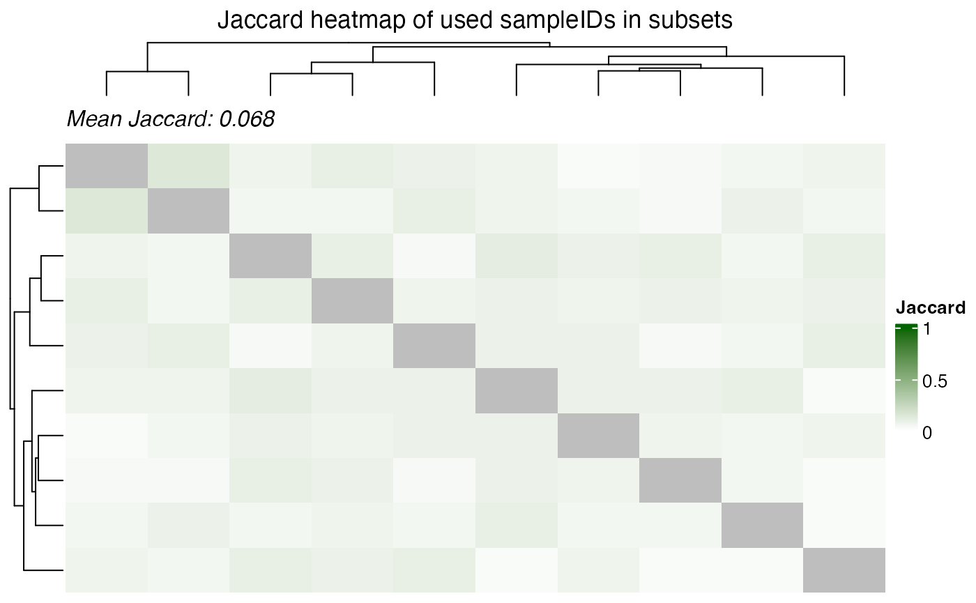
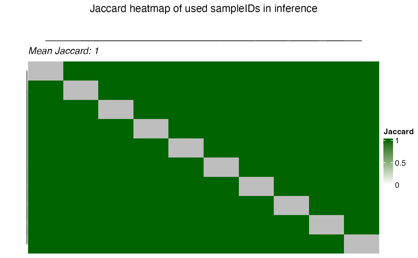
Histogram of p-values across iterations

Dependence of multiple subsets

From a biological view, feautures with low p-value across subsets are more likely to be true positives. However, from a statistical perspective, the p-values are not independent across subsets and hence to aggregate them it is important to consider. The samples are shared across the subsets and this sharing of samples can be visualized using the plot_jaccard_heatmap() function.

plot_jaccard_heatmap(
  data = combined_id,
  role = "X",
  title = "Jaccard heatmap of used sampleIDs in subsets",
)

plot_jaccard_heatmap(
  data = combined_id,
  role = "Y",
  title = "Jaccard heatmap of used sampleIDs in inference",
)

Jaccard heatmap

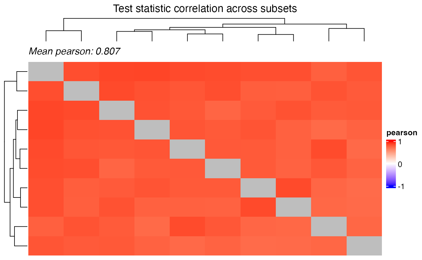
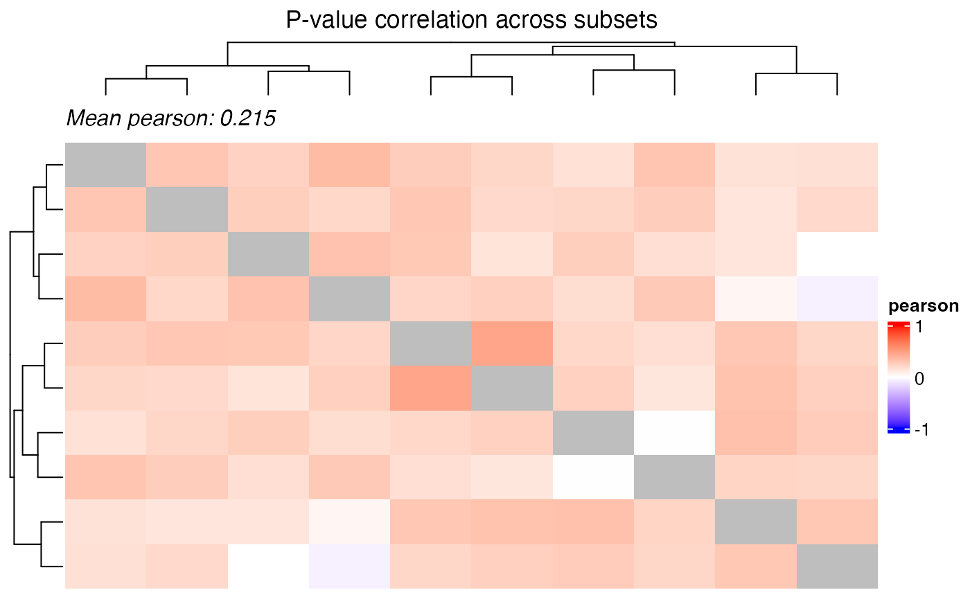
Correlation of the test statistic and the p-values can be visualized using the plot_correlation_heatmap() function.

plot_correlation_heatmap(
  data = combined_res,
  value_col = "T_obs",
  iter_col = "iteration",
  title = "Test statistic correlation across subsets",
)

plot_correlation_heatmap(
  data = combined_res,
  value_col = "p_value",
  iter_col = "iteration",
  title = "P-value correlation across subsets",
)

Correlation heatmap

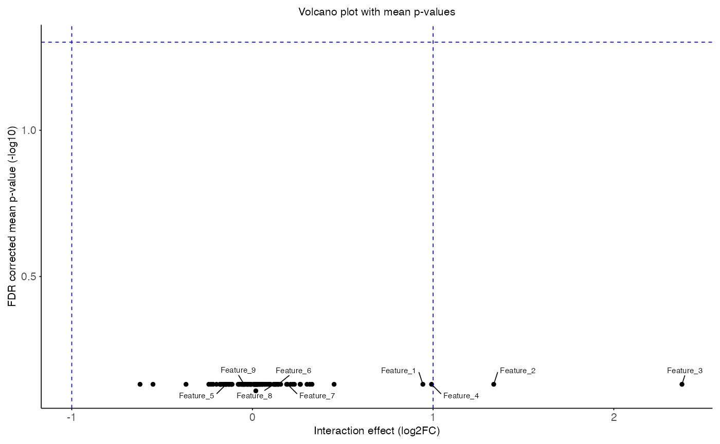
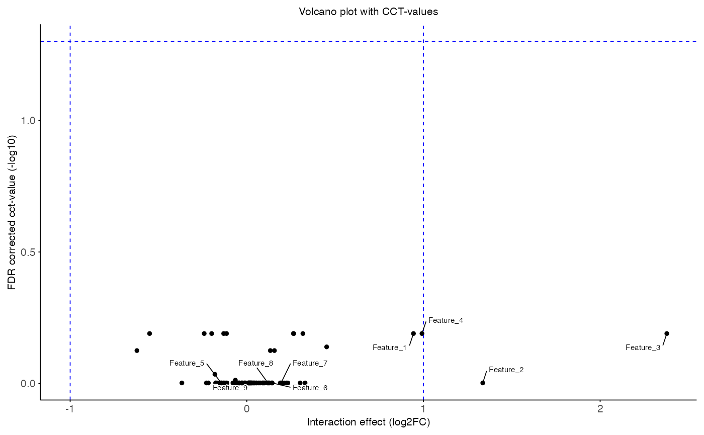
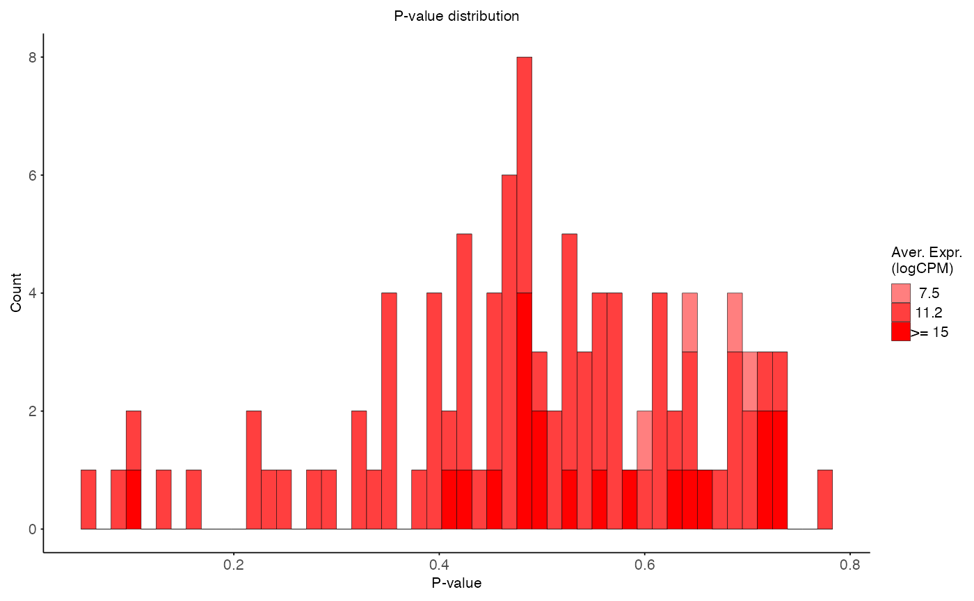
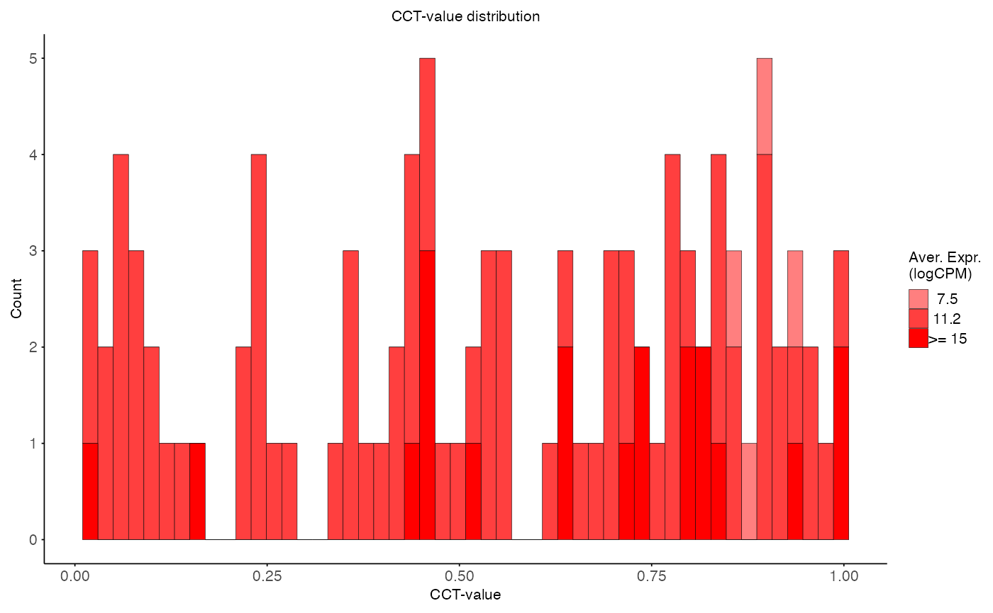
Aggregation of multiple subsets

To aggregate the p-values for each subset we decided on two methods one is simply taking the mean of the p-values. Another approach is to use a cauchy-combination test which is possible under abbretrary dependance. The function to call on multiple subsets is summarize_subsets().

# Aggregation of p-values
aggregated_res <- summarize_subsets(
  data = combined_res
)

print(head(aggregated_res))
#>     feature      T_obs    p_value    p_adj  cct_value   cct_adj prob_sig
#> 1 Feature_1  0.9433479 0.06121674 0.738991 0.04089120 0.6457288        0
#> 2 Feature_2  1.3356309 0.28316862 0.738991 0.21907536 0.9950796        0
#> 3 Feature_3  2.3774571 0.10392259 0.738991 0.05783392 0.6457288        0
#> 4 Feature_4  0.9913829 0.08259291 0.738991 0.05924215 0.6457288        0
#> 5 Feature_5 -0.1450369 0.40067978 0.738991 0.25437098 0.9950796        0
#> 6 Feature_6  0.1433863 0.63721534 0.738991 0.86123688 0.9950796        0
#>    ave_expr
#> 1 12.983109
#> 2 11.135611
#> 3 10.681342
#> 4 12.756946
#> 5 12.409589
#> 6  9.063243

plot_volcano(
  data = aggregated_res, 
  x_var = "T_obs", 
  y_var = "p_adj", 
  sig_thr = 0.05, 
  effect_thr = 1,
  features = head(interaction_res$feature, 9),
  title = "Volcano plot with mean p-values", 
  x_label = "Interaction effect (log2FC)",
  y_label = "FDR corrected mean p-value (-log10)"
)

plot_volcano(
  data = aggregated_res, 
  x_var = "T_obs", 
  y_var = "cct_adj", 
  sig_thr = 0.05, 
  effect_thr = 1,
  features = head(interaction_res$feature, 9),
  title = "Volcano plot with CCT-values", 
  x_label = "Interaction effect (log2FC)",
  y_label = "FDR corrected cct-value (-log10)"
)

plot_pvalue_distribution(
  data = aggregated_res,
  x_var = "p_value",
  fill_var = "ave_expr",
  facet_col = NULL,
  facet_levels = NULL,
  title = "P-value distribution",
  x_label = "P-value",
  y_label = "Count",
  fill_label = "Aver. Expr.\n(logCPM)"
)

plot_pvalue_distribution(
  data = aggregated_res,
  x_var = "cct_value",
  fill_var = "ave_expr",
  facet_col = NULL,
  facet_levels = NULL,
  title = "CCT-value distribution",
  x_label = "CCT-value",
  y_label = "Count",
  fill_label = "Aver. Expr.\n(logCPM)"
)

Two volcano plots