Permutation Correlation Difference

Introduction

While interaction effects are useful to test the effect of ancestry on single genes, correlation difference allows to look at a the global trend across all genes. The same subset approach is used to correct for the overrepresentation of EUR ancestry. This time the remaining Europeans are used as a reference or test set to test the correlation. In principle the idea is that the correlation (of effect sizes of the relationship) must be higher between the remaining Europeans and the EUR-subset than between the remaining Eurpeans and non-Europeans. Also in this case permutations are used to derive a null distribution in this case of the correlation differences between EUR-subset and the compared ancestry. This gives a estimate of the generalizability across all genes.

Data setup

library(CrossAncestryGenPhen)
library(ggplot2)

# Seed for reproducibility
seed <- 42  
set.seed(seed)

# Simulate example data
p <- 100  # Number of genes
n_EUR <- 600 
n_AFR <- 40  

# Expression matrices for EUR and AFR ancestries
X <- matrix(rnorm(n_EUR * p), nrow = n_EUR, ncol = p)
Y <- matrix(rnorm(n_AFR * p), nrow = n_AFR, ncol = p)
colnames(X) <- colnames(Y) <- paste0("Gene_", seq_len(p))

# Metadata for EUR and AFR ancestries
# EUR: overrepresented compared to AFR
MX <- data.frame(
  id = paste0("EUR_", seq_len(n_EUR)),
  condition = factor(c(rep("Control", 400), rep("Case", 200))),
  ancestry = "EUR"
)

# AFR: underrepresented compared to EUR
MY <- data.frame(
  id = paste0("AFR_", seq_len(n_AFR)),
  condition = factor(c(rep("Control", 10), rep("Case", 30))),
  ancestry = "AFR"
)

# Rownames of matrix must be smaple ids
rownames(X) <- MX$id
rownames(Y) <- MY$id

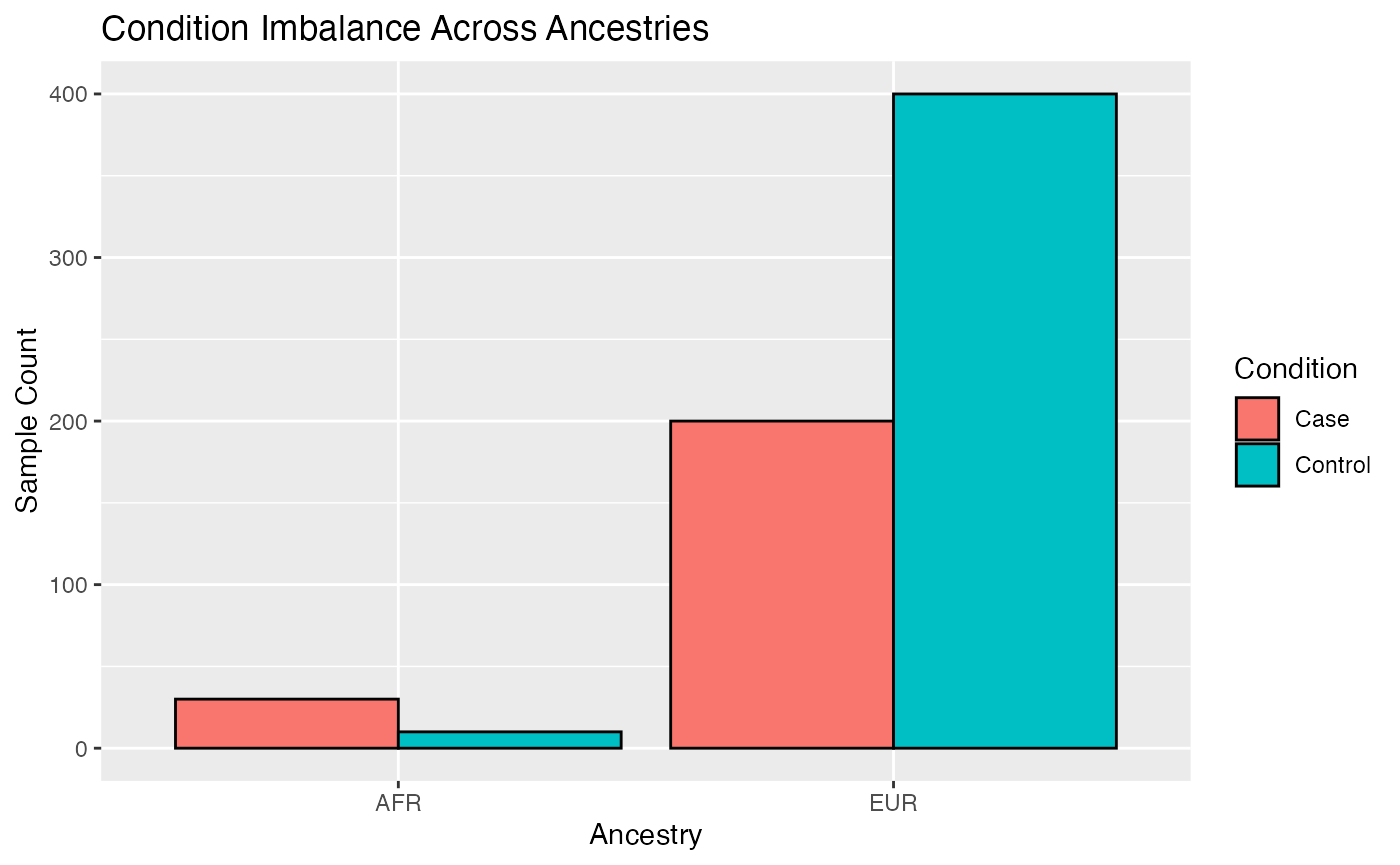
# Visualize sample size imbalance
meta <- rbind(MX, MY)

# Plot
ggplot(meta, aes(x = ancestry, fill = condition)) +
  geom_bar(position = "dodge", color = "black") +
  labs(
    title = "Condition Imbalance Across Ancestries",
    x = "Ancestry",
    y = "Sample Count",
    fill = "Condition"
  ) 

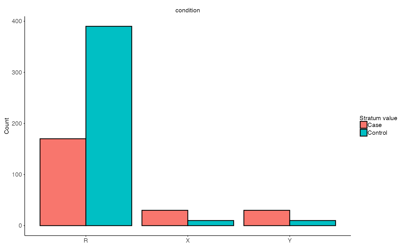
Single subset run of permutation correlation effect

The function perm_correlation_difference() calculates the correlation to the reference set

stratify_col <- "condition" # Column to stratify on

# Split the data into stratified sets
split <- split_stratified_ancestry_sets(
  X = X,
  Y = Y,
  MX = MX,
  MY = MY,
  g_col = stratify_col,
  seed = 42
)

# Visulaize stratified sets
plot_stratified_sets(
  MX = split$test$M,
  MY = split$inference$M,
  MR = split$train$M,
  g_col = stratify_col
)

# Permutation correlation difference 
B <- 100  # Number of permutations
method = "pearson" # Correlation coefficient

perm_res <- perm_correlation_difference(
  X = split$test$X,
  Y = split$inference$X,
  R = split$train$X,
  MX = split$test$M,
  MY = split$inference$M,
  MR = split$train$M,
  g_col = stratify_col,
  method = method,
  B = B, 
  seed = seed
)

str(perm_res)
#> List of 3
#>  $ summary_stats:'data.frame':   1 obs. of  6 variables:
#>   ..$ feature      : chr "Global"
#>   ..$ T_obs        : num 0.0748
#>   ..$ XR           : num -0.0108
#>   ..$ YR           : num 0.064
#>   ..$ p_param_value: num 0.591
#>   ..$ p_emp_value  : num 0.644
#>  $ T_null       : num [1:100, 1] -0.0121 0.1882 0.0257 0.1055 -0.0015 ...
#>   ..- attr(*, "dimnames")=List of 2
#>   .. ..$ : NULL
#>   .. ..$ : chr "T_null"
#>  $ B_used       : int 100

The output of the function contains three items:

1. summary_stats: Contains estimated difference in correlation (T_obs) and p_values per features. It also contains the correlation values to the reference XR and XY, respectively.

2. T_null: The observed null distribution for each feature across permutations.

3. B_used: The number of permutation iterations used to estimate the null distribution.